Category: Blog

Your blog category

  • The Ocean’s Plastic Is Rising Faster Than Our Knowledge of It

    The Ocean’s Plastic Is Rising Faster Than Our Knowledge of It

    Microplastics hero

    The world’s oceans are accumulating microplastics faster than we are building the knowledge needed to track them. That is the uncomfortable pattern in the NOAA NCEI Global Marine Microplastics Harmonized Database, which I analyzed: 29,076 observations spanning April 1972 to April 2026, drawn from every ocean basin. Within the most method-comparable subset of that record, median surface concentrations have risen roughly eighty-fold since the 2000s, yet 94% of all observations sit in the Northern Hemisphere, and the last eight years of “growth” in the database reflect a citizen-science beach survey rather than more open-ocean research.

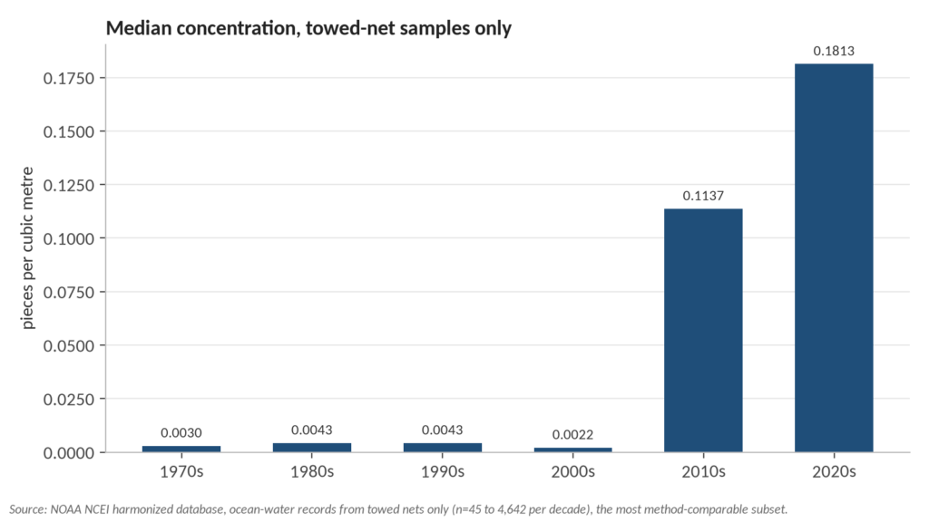
    TL;DR: Concentrations of surface microplastics in towed-net samples rose from about 0.002 pieces per cubic metre in the 2000s to 0.18 in the 2020s; sampling remains overwhelmingly concentrated in the Northern Hemisphere; and raw record counts after 2018 mostly measure a volunteer nurdle-survey program, not ocean conditions. The full analysis script, data, and charts are on GitHub.

    What the data actually is

    The NOAA NCEI harmonized database (NCEI Accession 0306475) is the largest openly available compilation of marine microplastic observations, updated quarterly and documented in Scientific Data. Each record is one measurement: where, when, what medium (ocean water, beach, sediment, or a nurdle survey), what method, and a concentration. Two properties shape everything that follows.

    First, it is presence-only data. A record means a sample was taken and plastic was counted; an area with no records may be pristine or simply unobserved. Second, the three units in the collection (pieces per cubic metre, pieces per 10 minutes of trawling, and pieces per kilogram of dry sediment) are not comparable, so any trend analysis must be restricted to one unit and, ideally, one family of methods.
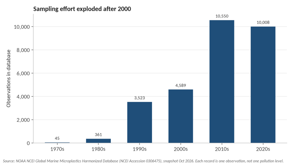
    sampling effort by decade

    The trend: flat, then a sharp rise

    Restricting the analysis to ocean-water samples collected with towed nets (neuston, manta, plankton, bongo and AVANI nets, the same technique family across five decades) shows medians that barely moved between the 1970s and the 2000s: 0.003, 0.0043, 0.0043 and 0.0022 pieces per cubic metre. Then the 2010s median jumps to 0.114 and the 2020s to 0.181, a roughly eighty-fold increase over the 2000s median, based on between 45 and 4,642 records per decade (see the analysis).
    concentration trend towed nets

    Honesty requires the caveat that this figure blends a real pollution signal with changes in how science looks: finer mesh sizes, more targeted expeditions into known accumulation zones, and better laboratory detection all push measured concentrations upward. But the direction is consistent with what production data predicts. Global plastics use was 460 million tonnes in 2019 and is projected to reach 1,231 million tonnes by 2060 according to the OECD, and models estimate rivers deliver roughly one million tonnes of plastic to the ocean each year, with more than 1,000 rivers responsible for 80% of that input (Meijer et al. 2021, Science Advances). The ocean had no trend toward less input at any point in this window.

    Where scientists look, and where they don’t

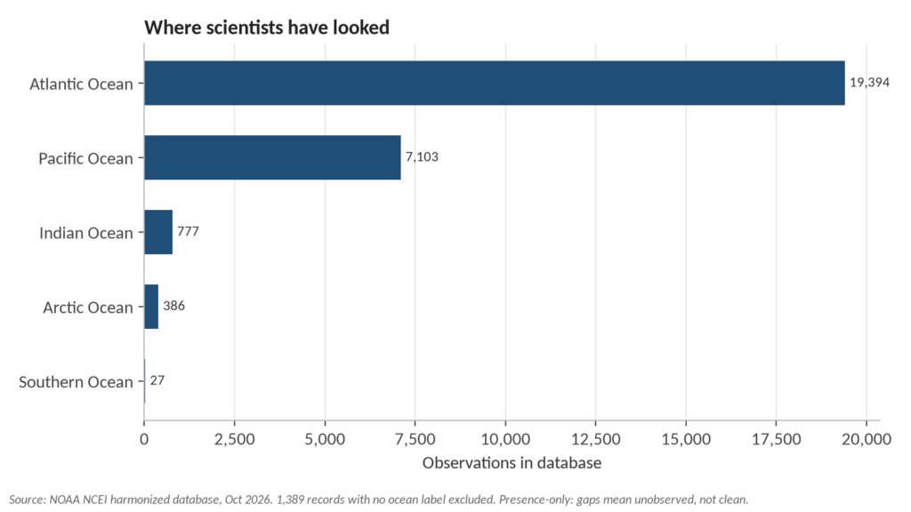
    Of 29,076 records, 94.1% sit north of the equator. The Southern Hemisphere’s share of annual observations peaked at about 13% in the 2010s and has fallen below 2% in the 2020s. The Indian Ocean, which borders some of the fastest-growing coastal populations on Earth, has 777 records. The Arctic has 386. The entire Southern Ocean, more than 20 million square kilometres, has 27.
    records by ocean

    This is not a conspiracy, it is expedition economics: research vessels, funding calls and graduate students cluster in Europe, North America and East Asia. But its consequence is a knowledge gap that maps onto global inequality. The coastal communities most dependent on fishing and most exposed to unmanaged plastic waste are among the least-sampled on the planet, so when a region’s waters are finally studied, findings often surprise: hotspots emerge where none were measured. In this database the South China Sea shows the highest regional median (about 1,001 pieces per cubic metre, from a focused 115-record campaign), followed by the Celtic Sea and the Mediterranean, while the Caribbean’s median of zero across 1,805 records mostly reflects how few targeted campaigns looked there, not clean water.

    The trap in rising bar charts

    A naive chart of records per year shows apparent “growth” after 2018 that is entirely an artifact. From 2019 onward, more than half of all new records come from Nurdle Patrol, a citizen-science program that counts pre-production plastic pellets on beaches in ten-minute surveys, recorded in its own unit. Dedicated open-ocean water-column records, meanwhile, fall from over 1,100 in 2015 to zero in 2025 and 2026 so far. Anyone quoting the database’s rising record count as evidence of rising pollution is measuring the birth of a volunteer program. The reverse also matters: the disappearance of professional open-ocean sampling from the most recent years means the trend analysis above rests on an aging data stream.
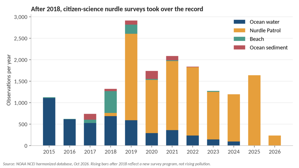
    Chart4 records by medium 2015

    Why this is a climate story

    Microplastics are where the plastic crisis and the climate crisis physically meet. In the Arctic, sea ice acts as a conveyor and a time capsule: it traps particles as it forms and releases them as it melts, and melting ice is simultaneously opening the region to more shipping and fishing, themselves local sources of plastic debris (NOAA Arctic Report Card; Mountford et al. 2021). Researchers have measured concentrations exceeding 12,000 particles per litre in some Arctic sea ice (The Guardian, 2018), orders of magnitude above anything in this surface-water database, in a region with 386 records in fifty-four years. And the particles are not staying remote: a 2022 study detected plastic in the blood of 17 of 22 human donors (Leslie et al., Environment International).

    Meanwhile the policy machinery is stalling. Talks toward a global plastics treaty collapsed in Geneva in August 2025 and, a year on, the process remains deadlocked, with the next real test not expected before late 2026 (Health Policy Watch, August 2026; World Economic Forum, August 2025). A treaty that cuts production upstream would address the cause; a data gap that keeps the least-sampled regions unmeasured would otherwise stay invisible while the problem compounds.

    What the record itself argues for

    Three things follow directly from this analysis. First, treat raw observation counts in any environmental database as evidence about observation, and decompose them by method, medium and unit before quoting them as trends. Second, the fastest way to close the knowledge gap is not new instrumentation but new sampling agreements that put research capacity in the hands of institutions in the Global South, whose waters the Southern Hemisphere gap leaves dark. Third, citizen science earns its place here: the nurdle surveys are genuine data, but they belong to their own unit and question, and mixing them into open-ocean trends corrupts both.

    FAQ

    Does this dataset show ocean plastic pollution is getting worse? Within the comparable towed-net subset, yes: median measured concentrations rose roughly eighty-fold from the 2000s to the 2020s. Part of that rise reflects better detection and targeted sampling, so the honest statement is that nothing in the record suggests a decline, and the measured signal points upward.

    Why is the Southern Hemisphere so underrepresented? Research funding, vessel availability and academic networks concentrate in the Northern Hemisphere. The database mirrors that: 94% of records are north of the equator, and the Southern Hemisphere’s share of annual observations has fallen below 2% in the 2020s.

    Can I reproduce this analysis? Yes. The dataset snapshot, the base-R script, and all summary tables are in the GitHub repository. The script needs no packages and runs in about a minute. Method summary: the dataset was split by medium and unit, and the trend reported here uses only ocean-water records in pieces per cubic metre collected with towed nets, aggregated as medians by decade; per-decade record counts in that subset run from 45 in the 1970s to 4,642 in the 2010s.

    What are nurdles? Pre-production plastic pellets, the raw material of the plastics industry. They spill in transit and handling, accumulate on shorelines, and are the subject of the Nurdle Patrol citizen surveys that dominate the database’s recent records.

    What would the global plastics treaty change? Negotiations aim at a legally binding instrument covering the plastic lifecycle, including marine environments, but talks collapsed in Geneva in August 2025 without agreement, and remain stalled as of late 2026. Without upstream production cuts, models project plastics use tripling by 2060 (OECD Global Plastics Outlook, 2022).

    Reproducibility. The dataset snapshot, the base-R analysis script, and all summary tables are in the GitHub repository. Analysis and writing: Qanit Takmeel.

  • Predicting Diabetes: Comparing Logistic Regression, SVMs, and Random Forests

    While exploring Kaggle’s vast data science resources, I discovered an intriguing diabetes dataset and decided to develop a predictive model. The dataset structure is elegantly simple, featuring 8 independent variables and a target variable called Outcome, which identifies the presence or absence of diabetes. My objective is to create a robust model that can accurately predict diabetes based on these variables.

    Dataset Overview

    This comprehensive medical dataset contains diagnostic measurements specifically collected for diabetes prediction based on various health indicators. It encompasses 768 female patient records, with each record containing 8 distinct health parameters. The Outcome variable serves as the binary classifier, indicating diabetes presence (1) or absence (0). This dataset serves as an excellent resource for training and evaluating machine learning classification models in the context of diabetes prediction.

    • Pregnancies (Integer): Total pregnancy count for each patient.
    • Glucose (Integer): Post 2-hour oral glucose tolerance test plasma concentration (mg/dL).
    • BloodPressure (Integer): Measured diastolic blood pressure (mm Hg).
    • SkinThickness (Integer): Measured triceps skin fold thickness (mm).
    • Insulin (Integer): Measured 2-hour serum insulin levels (mu U/ml).
    • BMI (Float): Calculated body mass index using weight(kg)/height(m)^2.
    • DiabetesPedigreeFunction (Float): Calculated genetic diabetes predisposition score based on family history.
    • Age (Integer): Patient’s age in years.
    • Outcome (Binary): Target variable indicating diabetes (1) or no diabetes (0).

    This valuable dataset, adapted from the National Institute of Diabetes and Digestive and Kidney Diseases (NIDDK), is frequently utilized in data science research focusing on healthcare analytics and medical diagnostics.

    Exploratory Data Analysis

    Initial data examination reveals a significant concern: multiple variables including Blood Pressure, Glucose, Skin Thickness, Insulin, and BMI contain zero values. These likely represent measurement errors, necessitating their removal for accurate analysis.

    diabetes <- read.csv('diabetes_dataset.csv') #Read Data
    summary(diabetes)
    Diabetes Summary

    Post removal of zero values, our dataset reduces to 392 observations. Though smaller, this sample size remains adequate for developing a reliable predictive model.

    diabetes <- diabetes %>%
      filter(BloodPressure != 0) %>%
      filter(Glucose != 0) %>%
      filter(SkinThickness != 0) %>%
      filter(Insulin != 0) %>%
      filter(BMI != 0)
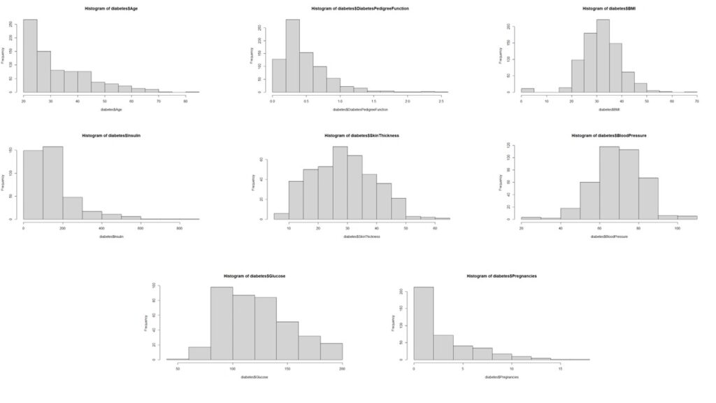
    hist(diabetes$Age)
    hist(diabetes$DiabetesPedigreeFunction)
    hist(diabetes$BMI)
    hist(diabetes$Insulin)
    hist(diabetes$SkinThickness)
    hist(diabetes$BloodPressure)
    hist(diabetes$Glucose)
    hist(diabetes$Pregnancies)
    Histograms

    Subsequently, we analyze the distribution patterns of all independent variables.

    The analysis reveals that most variables, except pregnancy, age, and insulin, deviate from normal distribution. The non-normal distribution of pregnancy data aligns with logical expectations.

    Data Preprocessing

    We implement these specific transformations:

    • Insulin: Box-Cox Transform
    • Age: Box-Cox Transform
    • Age: Square Root Transform
    #PreProcess Data to Get everything into Normal Distribution
    
    #Applying Box-Cox Transform on Age
    
    boxcox(diabetes$Age ~ 1)
    diabetes$boxcoxAge <- (diabetes$Age^-1.4 - 1)/-1.4
    hist(diabetes$boxcoxAge)
    
    #Applying Box-Cox Transform on Insulin
    
    boxcox(diabetes$Insulin ~ 1)
    diabetes$boxcoxInsulin <- (diabetes$Insulin^0.05 -1)/0.05
    hist(diabetes$boxcoxInsulin)
    
    #Applying Box-Cox Transform on Pregnancies
    diabetes$Pregnancies
    diabetes$sqrtPregnancies <- sqrt(diabetes$Pregnancies)
    hist(diabetes$sqrtPregnancies)

    Finally, we apply max-min scaling to normalize all values between 0 and 1, effectively preventing any data artifacts from influencing our analysis.

    #Storing relevant variables in a new dataframe and scaling the data
    
    diabetes.clean <- diabetes %>%
      dplyr::select(
        Outcome,
        DiabetesPedigreeFunction,
        sqrtPregnancies,
        SkinThickness,
        boxcoxInsulin,
        boxcoxAge,
        BMI,
        Glucose,
        BloodPressure
      )
      
    
    preproc <- preProcess(diabetes.clean, method = "range")
    scaled.diabetes.clean <- predict(preproc, diabetes.clean)
    
    head(scaled.diabetes.clean)
    str(scaled.diabetes.clean)
    scaled.diabetes.clean$Outcome <- as.factor(scaled.diabetes.clean$Outcome)
    

    Looking for correlations in the variables

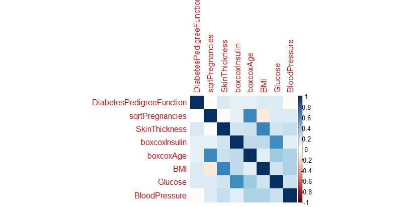
    Upon analyzing the correlation matrix, the data science analysis reveals minimal significant correlations among the variables, suggesting we can proceed with treating them as independent predictors in our modeling approach.

    # Looking for Correlations within the Data
    
    num.cols <- sapply(scaled.diabetes.clean, is.numeric)
    cor.data <- cor(scaled.diabetes.clean[,num.cols])
    cor.data
    corrplot(cor.data, method = 'color')
    Corrplot

    Splitting the data into training and testing set

    For model development and evaluation, we implement a standard data partitioning strategy, allocating 70% of the observations to the training dataset and reserving the remaining 30% for testing purposes.

    #Splitting Data into train and test sets
    
    sample <- sample.split(scaled.diabetes.clean$Outcome, SplitRatio = 0.7)
    train = subset(scaled.diabetes.clean, sample == TRUE)
    test = subset(scaled.diabetes.clean, sample == FALSE)

    Building a Model

    Our predictive modeling approach incorporates three distinct machine learning techniques: Logistic Regression, Support Vector Machines, and Random Forests.

    Logistic Regression

    The logistic regression implementation yields a respectable accuracy of 77.12%. The model identifies Age, BMI, and Glucose as significant predictors of diabetes, with the diabetes pedigree function showing moderate influence. This suggests that while genetic predisposition plays a role, lifestyle factors remain crucial in diabetes prevention.

    Support Vector Machines

    Despite parameter tuning efforts, the Support Vector Machines algorithm demonstrates slightly lower performance, achieving 74.9% accuracy compared to the logistic regression model.

    Random Forest

    Random Forests emerge as the superior performer among the three approaches, delivering the highest accuracy at 79.56%.

    A critical observation across all models is the notably lower proportion of Type I errors. In this medical context, false negatives pose a greater risk than false positives, making this characteristic particularly relevant.

    Comparing the Models

    A comparative analysis of model performance metrics reveals Random Forests as the top performer, though there remains room for improvement. It’s worth noting that the necessity to exclude numerous observations due to measurement inconsistencies may have impacted model performance. While this model shows promise as a preliminary diabetes screening tool with reasonable accuracy, developing a more precise predictive model would require additional data points and refined measurements.

    Code

    ### LOGISTIC REGRESSION ###
    
    log.model <- glm(formula=Outcome ~ . , family = binomial(link='logit'),data = train)
    summary(log.model)
    fitted.probabilities <- predict(log.model,newdata=test,type='response')
    fitted.results <- ifelse(fitted.probabilities > 0.5,1,0)
    misClasificError <- mean(fitted.results != test$Outcome)
    print(paste('Accuracy',1-misClasificError))
    table(test$Outcome, fitted.probabilities > 0.5)
    
    ### SVM ####
    
    svm.model <- svm(Outcome ~., data = train)
    summary(svm.model)
    predicted.svm.Outcome <- predict(svm.model, test)
    table(predicted.svm.Outcome, test[,1])
    tune.results <- tune(svm, 
                         train.x = train[2:9], 
                         train.y = train[,1], 
                         kernel = 'radial',
                         ranges = list(cost=c(1.25, 1.5, 1.75), gamma = c(0.25, 0.3, 0.35)))
    summary(tune.results)
    tuned.svm.model <- svm(Outcome ~., 
                           data = train, 
                           kernel = "radial",
                           cost = 1.25,
                           gamma = 0.25,
                           probability = TRUE)
    summary(tuned.svm.model)
    print(svm.model)
    tuned.predicted.svm.Outcome <- predict(tuned.svm.model, test)
    table(tuned.predicted.svm.Outcome, test[,1])
    Table

  • Are US Police Trigger Happy?

    Recently, I stumbled upon a Washington Post article discussing the statistics of police-involved shootings and fatalities over recent years. The article referenced a comprehensive dataset, which I managed to download before encountering the paywall. This dataset documented all fatal police shootings spanning roughly a decade. While the data extended into 2024, I’ve excluded those entries from my analysis since the year is still ongoing.

    The dataset contained several key parameters:

    1. Date
    2. Name
    3. Age
    4. Gender
    5. Armed
    6. Race
    7. City
    8. State
    9. Flee
    10. Body Camera
    11. Signs of Mental Illness
    12. Police Departments Involved

    The dataset revealed a staggering 9893 cases – an alarmingly high number of individuals who lost their lives without due process, regardless of their alleged criminal activities. Each number represents a person denied their constitutional right to a fair trial.

    After examining the data quality and addressing missing values across various columns, I had to exclude approximately 400 entries, leaving me with 9509 cases for analysis. This sample size remains statistically significant enough to draw meaningful conclusions about the patterns present in the overall dataset.

    Demographics of the Victims

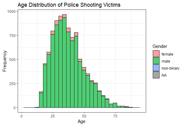
    My initial analysis focused on examining the age distribution of police shooting victims. The data showed a concentration in the 25-60 age range, which aligns with general crime statistics. This age group typically shows higher involvement in criminal activities or presence in high-crime areas.

    Agedistribution

    Further investigation revealed interesting patterns when analyzing racial demographics.

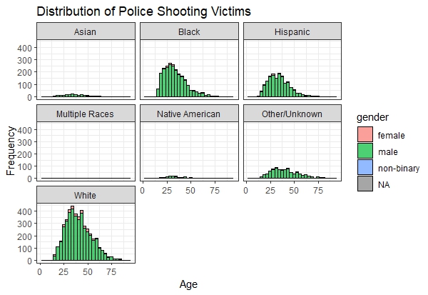
    The data initially appears to reflect expected proportions, given that White Americans comprise roughly 65-70% of the total population, explaining their higher representation among police shooting victims. However, a deeper analysis reveals concerning trends: Black and Hispanic victims show a notably skewed age distribution toward younger ages, with victims predominantly in their late teens and early twenties. In contrast, White victims follow a more normal distribution pattern, typically falling in their late twenties or thirties. This raises questions about whether social changes over the past few decades have led to increased police interactions with younger people of color. While this observation warrants further investigation, additional data would be needed to draw definitive conclusions about these demographic disparities.

    Age Distribution Based On Race

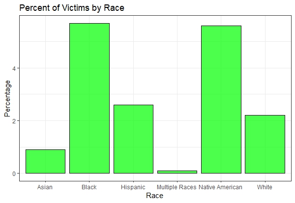
    While raw numbers provide one perspective, examining the percentage of population affected by police interactions offers deeper insights. I analyzed the Washington Post dataset in conjunction with US demographic data (sourced from here) to calculate these proportional impacts.

    Percentofvictimsbyrace

    In my analysis, I excluded the “Unknown” race category due to the discrepancy between census data accuracy and the Washington Post dataset’s limitations, likely stemming from incomplete police documentation. It’s worth noting that approximately 10% of victims in the original dataset had unspecified racial classifications.

    The proportional analysis reveals striking disparities: Native American and Black populations face double the likelihood of fatal police encounters compared to white populations. Hispanic individuals experience similar rates of fatal police interactions as white populations, while Asian Americans show half the likelihood of such encounters. The “Multiple Races” category contained insufficient data points for meaningful analysis, possibly due to inconsistent reporting in police records.

    One potential explanation for Asian Americans’ lower representation in police shooting statistics could be their generally reduced frequency of police interactions. While Asian Americans are widely recognized as one of America’s most successful immigrant groups, their family structure, as documented in Pew Research findings, might be a contributing factor. However, this remains a preliminary hypothesis requiring further investigation for definitive conclusions.

    Mental Health of the Victims

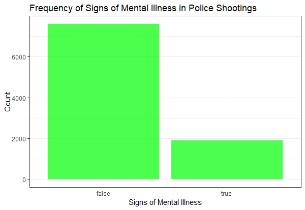
    My analysis then shifted to examining the mental health status of victims.

    The findings are concerning: approximately 2,000 victims over the past decade exhibited signs of mental illness. This suggests that redirecting resources toward mental health professionals and social workers might be more effective than relying solely on law enforcement.

    Mentalhealth

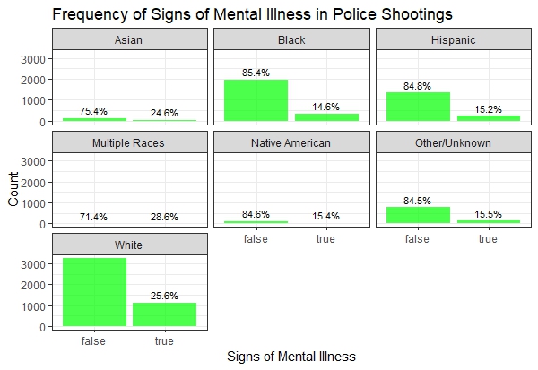
    Breaking down mental health data by race reveals another pattern: white victims of police shootings are roughly three times more likely to be classified as not mentally ill, while Black, Hispanic, and Native American victims show a five-to-one ratio between those classified as not mentally ill versus those showing signs of mental illness.

    Mentalinessbyrace

    It’s crucial to note that these mental health classifications are based on behavioral signs observed during police encounters, rather than professional diagnoses or established medical histories.

    Circumstantial Trends

    I focused on two key situational factors:

    1. Whether the victims were trying to flee?
    2. Whether the victims were armed?

    Were the Victims trying to Flee?

    Fleeing Behavior

    Analysis across racial demographics indicates that approximately half of the victims were not attempting to escape during their encounters with law enforcement. This suggests that many victims were likely complying with police directives, though definitive conclusions cannot be drawn solely from this dataset.

    Fleeingmode

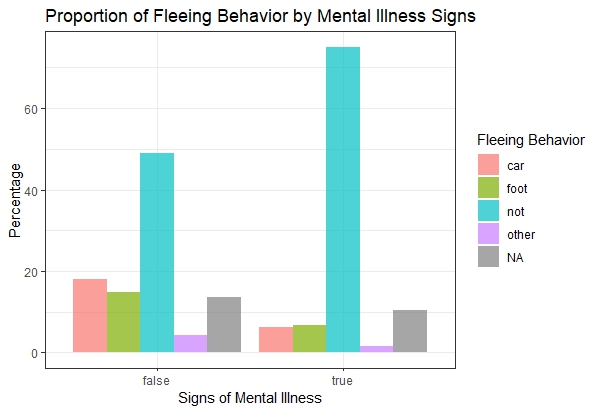
    When examining the intersection of mental health status and escape attempts, a notable pattern emerges: the majority of mentally ill victims were not attempting to flee. This observation raises significant concerns about the necessity of lethal force in situations where alternative intervention methods might have been viable.

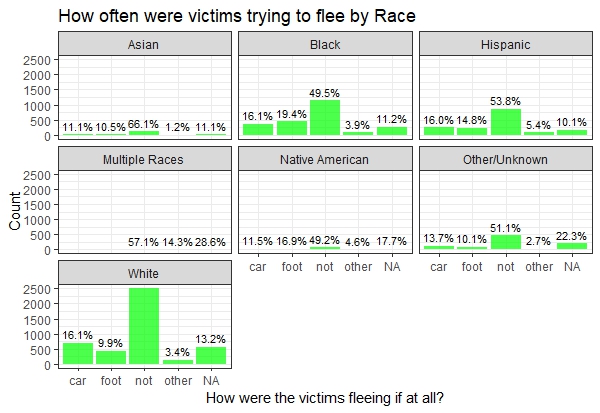
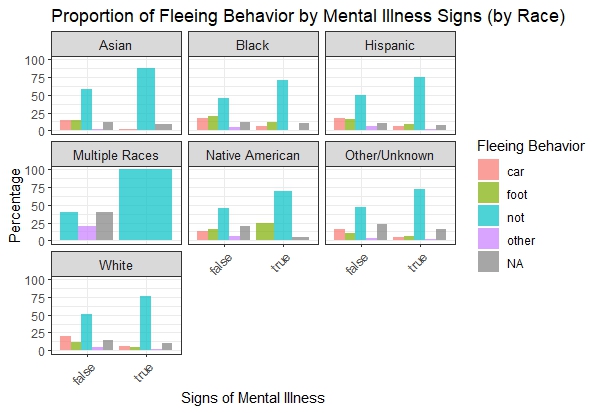
    The behavioral patterns of victims, when analyzed across different racial groups, demonstrate remarkable consistency. Where sufficient data exists, the distribution of victim responses appears uniform across racial categories, suggesting that behavioral responses to police encounters transcend racial boundaries.

    Fleeingbehaviorbyrace

    This consistency prompts a critical inquiry: In cases where victims showed no intention to escape, what circumstances prevented successful arrests without resorting to lethal force?

    Were the Victims armed?

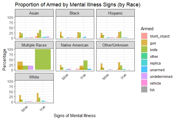
    Analysis of weapon possession among victims reveals firearms as the predominant type of armament. However, a distinct pattern emerges among mentally ill victims within Native American and Hispanic communities, where knife possession was notably more prevalent.

    Werevictimsarmed

    This finding underscores the potential benefits of enhanced firearm regulation in protecting law enforcement officers – a measure that has faced consistent opposition from the National Rifle Association.

    How have Police Shootings trended over time?

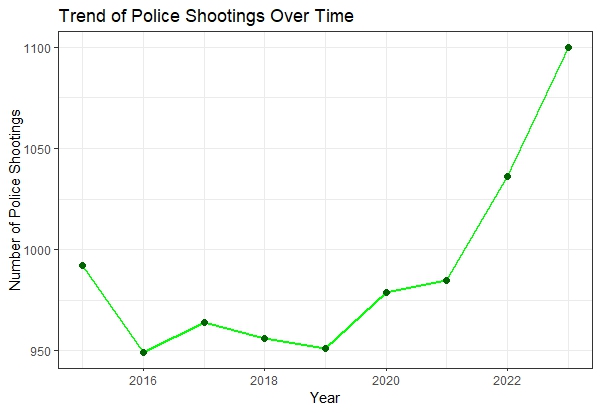
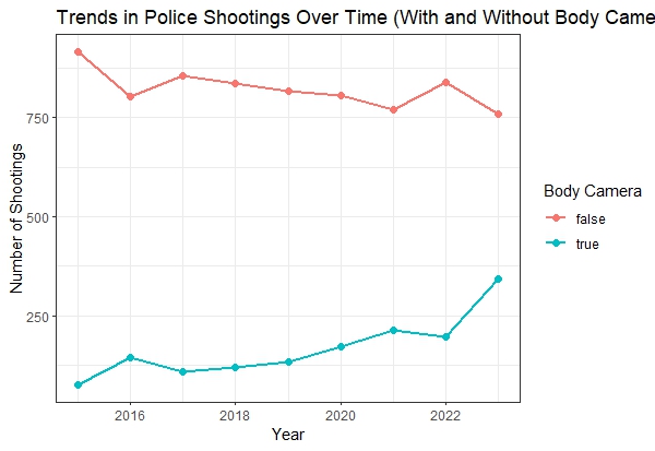
    The past decade has witnessed a concerning upward trajectory in police-involved shootings and resultant fatalities. While a ten-year span might seem relatively brief in historical context, the data reveals a disturbing average of approximately 1,000 victims annually.

    Trendovertime

    The implementation of body-worn cameras appears to have limited impact, though it’s important to acknowledge potential delays between policy implementation and observable outcomes.

    Bodycamera

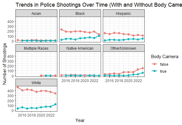
    Particularly concerning is the fact that body cameras were present in only one-third of documented cases.

    Bodycamwithrace

    When analyzing body camera usage across racial categories, while overall utilization shows an increasing trend, the data suggests a concerning pattern: incidents involving body cameras correlate with decreased likelihood of racial identification in victim documentation.

    Conclusion

    While numerous aspects of this issue warrant further investigation, certain data points remain unavailable – notably, comprehensive information about all police interactions, as this dataset exclusively covers fatal encounters.

    Nevertheless, the loss of 10,000 lives over a decade, through police shootings, represents an alarming figure, particularly considering that 20% of victims displayed signs of mental illness, and roughly half were not attempting to flee.

    This analysis, while revealing, highlights the need for more comprehensive research and complete datasets to fully understand and address these critical issues.

  • Spreadsheets: Common man’s programming tool

    #include <stdio.h>
    
    int main() {
        printf("Hello, World!\n");
        return 0;
    }

    I remember sitting in my computer science class about two decades ago and my teacher teaching us how to print “Hello World”. I never became a computer scientist – nor did I become a professional programmer. But I did come to appreciate how useful programming is for most professions.

    As an experimental Materials Scientist, I use programming so often to manipulate data, to analyze data, to predict the best possible set of experiments to run – and all the while I often wonder, why the common student is taught the dry programming of Hello World, that comes with C or C++ or Python or any of the other programming languages that exist, and why students are not introduced to the power of spreadsheets. Don’t get me wrong, I don’t undermine the value of true programming languages, but in my mind, =SUM(A1:A45) has more value than printf("Hello, World!\n"); as they offer a more practical entry point. Spreadsheets may not be sexy, but for most, they’re the perfect tool – since they can reduce errors, increase automation thereby, saving time.

    Here are a few good reasons why I feel spreadsheets are quite important:

    1. Low barrier to Entry
    2. Democratization of data
    3. WYSIWYG
    4. Teaching the fundamentals of programming

    And once someone graduates past the basic spreadsheet like Microsoft Excel, then they can even access VBA (a built-in programming language within excel) or Google Apps Script (a built in programming language within Google Sheets) to enable more complex functionalities.

    Spreadsheets offer a powerful and versatile toolset for anyone who works with data. Their low barrier to entry makes them accessible, while features like formulas and conditional formatting automate tasks, saving time and reducing errors. But spreadsheets hold a hidden gem: VBA in Excel and Apps Script in Google Sheets. These built-in programming languages unlock a whole new level of automation and functionality. Imagine automating complex data analysis, generating reports with a single click, or creating custom functions tailored to your specific needs.

    The next time you find yourself drowning in data, don’t underestimate the power of your spreadsheet. With a little exploration and the help of readily available online resources, you can unlock the hidden potential of VBA or Apps Script and transform your workflow. So, ditch the “Hello World” and dive into the world of spreadsheet programming – the possibilities are endless!