While exploring Kaggle’s vast data science resources, I discovered an intriguing diabetes dataset and decided to develop a predictive model. The dataset structure is elegantly simple, featuring 8 independent variables and a target variable called Outcome, which identifies the presence or absence of diabetes. My objective is to create a robust model that can accurately predict diabetes based on these variables.
Dataset Overview
This comprehensive medical dataset contains diagnostic measurements specifically collected for diabetes prediction based on various health indicators. It encompasses 768 female patient records, with each record containing 8 distinct health parameters. The Outcome variable serves as the binary classifier, indicating diabetes presence (1) or absence (0). This dataset serves as an excellent resource for training and evaluating machine learning classification models in the context of diabetes prediction.
- Pregnancies (Integer): Total pregnancy count for each patient.
- Glucose (Integer): Post 2-hour oral glucose tolerance test plasma concentration (mg/dL).
- BloodPressure (Integer): Measured diastolic blood pressure (mm Hg).
- SkinThickness (Integer): Measured triceps skin fold thickness (mm).
- Insulin (Integer): Measured 2-hour serum insulin levels (mu U/ml).
- BMI (Float): Calculated body mass index using weight(kg)/height(m)^2.
- DiabetesPedigreeFunction (Float): Calculated genetic diabetes predisposition score based on family history.
- Age (Integer): Patient’s age in years.
- Outcome (Binary): Target variable indicating diabetes (1) or no diabetes (0).
This valuable dataset, adapted from the National Institute of Diabetes and Digestive and Kidney Diseases (NIDDK), is frequently utilized in data science research focusing on healthcare analytics and medical diagnostics.
Exploratory Data Analysis
Initial data examination reveals a significant concern: multiple variables including Blood Pressure, Glucose, Skin Thickness, Insulin, and BMI contain zero values. These likely represent measurement errors, necessitating their removal for accurate analysis.
diabetes <- read.csv('diabetes_dataset.csv') #Read Data
summary(diabetes)
Post removal of zero values, our dataset reduces to 392 observations. Though smaller, this sample size remains adequate for developing a reliable predictive model.
diabetes <- diabetes %>%
  filter(BloodPressure != 0) %>%
  filter(Glucose != 0) %>%
  filter(SkinThickness != 0) %>%
  filter(Insulin != 0) %>%
  filter(BMI != 0)
hist(diabetes$Age)
hist(diabetes$DiabetesPedigreeFunction)
hist(diabetes$BMI)
hist(diabetes$Insulin)
hist(diabetes$SkinThickness)
hist(diabetes$BloodPressure)
hist(diabetes$Glucose)
hist(diabetes$Pregnancies)
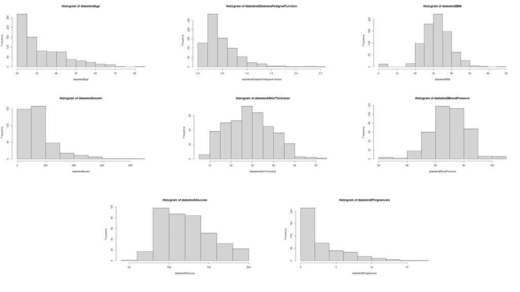
Subsequently, we analyze the distribution patterns of all independent variables.
The analysis reveals that most variables, except pregnancy, age, and insulin, deviate from normal distribution. The non-normal distribution of pregnancy data aligns with logical expectations.
Data Preprocessing
We implement these specific transformations:
- Insulin: Box-Cox Transform
- Age: Box-Cox Transform
- Age: Square Root Transform
#PreProcess Data to Get everything into Normal Distribution

#Applying Box-Cox Transform on Age

boxcox(diabetes$Age ~ 1)
diabetes$boxcoxAge <- (diabetes$Age^-1.4 - 1)/-1.4
hist(diabetes$boxcoxAge)

#Applying Box-Cox Transform on Insulin

boxcox(diabetes$Insulin ~ 1)
diabetes$boxcoxInsulin <- (diabetes$Insulin^0.05 -1)/0.05
hist(diabetes$boxcoxInsulin)

#Applying Box-Cox Transform on Pregnancies
diabetes$Pregnancies
diabetes$sqrtPregnancies <- sqrt(diabetes$Pregnancies)
hist(diabetes$sqrtPregnancies)
Finally, we apply max-min scaling to normalize all values between 0 and 1, effectively preventing any data artifacts from influencing our analysis.
#Storing relevant variables in a new dataframe and scaling the data

diabetes.clean <- diabetes %>%
  dplyr::select(
    Outcome,
    DiabetesPedigreeFunction,
    sqrtPregnancies,
    SkinThickness,
    boxcoxInsulin,
    boxcoxAge,
    BMI,
    Glucose,
    BloodPressure
  )


preproc <- preProcess(diabetes.clean, method = "range")
scaled.diabetes.clean <- predict(preproc, diabetes.clean)

head(scaled.diabetes.clean)
str(scaled.diabetes.clean)
scaled.diabetes.clean$Outcome <- as.factor(scaled.diabetes.clean$Outcome)
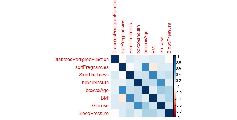
Looking for correlations in the variables
Upon analyzing the correlation matrix, the data science analysis reveals minimal significant correlations among the variables, suggesting we can proceed with treating them as independent predictors in our modeling approach.
# Looking for Correlations within the Data

num.cols <- sapply(scaled.diabetes.clean, is.numeric)
cor.data <- cor(scaled.diabetes.clean[,num.cols])
cor.data
corrplot(cor.data, method = 'color')
Splitting the data into training and testing set
For model development and evaluation, we implement a standard data partitioning strategy, allocating 70% of the observations to the training dataset and reserving the remaining 30% for testing purposes.
#Splitting Data into train and test sets

sample <- sample.split(scaled.diabetes.clean$Outcome, SplitRatio = 0.7)
train = subset(scaled.diabetes.clean, sample == TRUE)
test = subset(scaled.diabetes.clean, sample == FALSE)
Building a Model
Our predictive modeling approach incorporates three distinct machine learning techniques: Logistic Regression, Support Vector Machines, and Random Forests.
Logistic Regression
The logistic regression implementation yields a respectable accuracy of 77.12%. The model identifies Age, BMI, and Glucose as significant predictors of diabetes, with the diabetes pedigree function showing moderate influence. This suggests that while genetic predisposition plays a role, lifestyle factors remain crucial in diabetes prevention.
Support Vector Machines
Despite parameter tuning efforts, the Support Vector Machines algorithm demonstrates slightly lower performance, achieving 74.9% accuracy compared to the logistic regression model.
Random Forest
Random Forests emerge as the superior performer among the three approaches, delivering the highest accuracy at 79.56%.
A critical observation across all models is the notably lower proportion of Type I errors. In this medical context, false negatives pose a greater risk than false positives, making this characteristic particularly relevant.
Comparing the Models
A comparative analysis of model performance metrics reveals Random Forests as the top performer, though there remains room for improvement. It’s worth noting that the necessity to exclude numerous observations due to measurement inconsistencies may have impacted model performance. While this model shows promise as a preliminary diabetes screening tool with reasonable accuracy, developing a more precise predictive model would require additional data points and refined measurements.
Code
### LOGISTIC REGRESSION ###

log.model <- glm(formula=Outcome ~ . , family = binomial(link='logit'),data = train)
summary(log.model)
fitted.probabilities <- predict(log.model,newdata=test,type='response')
fitted.results <- ifelse(fitted.probabilities > 0.5,1,0)
misClasificError <- mean(fitted.results != test$Outcome)
print(paste('Accuracy',1-misClasificError))
table(test$Outcome, fitted.probabilities > 0.5)

### SVM ####

svm.model <- svm(Outcome ~., data = train)
summary(svm.model)
predicted.svm.Outcome <- predict(svm.model, test)
table(predicted.svm.Outcome, test[,1])
tune.results <- tune(svm,
                     train.x = train[2:9],
                     train.y = train[,1],
                     kernel = 'radial',
                     ranges = list(cost=c(1.25, 1.5, 1.75), gamma = c(0.25, 0.3, 0.35)))
summary(tune.results)
tuned.svm.model <- svm(Outcome ~.,
                       data = train,
                       kernel = "radial",
                       cost = 1.25,
                       gamma = 0.25,
                       probability = TRUE)
summary(tuned.svm.model)
print(svm.model)
tuned.predicted.svm.Outcome <- predict(tuned.svm.model, test)
table(tuned.predicted.svm.Outcome, test[,1])
Leave a Reply