Mastering XLOOKUP: The Ultimate Lookup Function for Scientists and Engineers

Oftentimes, data is stored in tables and frequently needs to be accessed. Take, for example, this data set (taken from kaggle.com) that lists the refractive indices of glass as a function of the percentage of the various elements present in it.

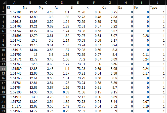
Imagine needing to quickly look up the elements of a glass with a particular refractive index. In older versions of Excel, you would use the VLOOKUP or INDEX and MATCH functions. However, with the powerful addition of the XLOOKUP function, these older functions are now largely obsolete.

Understanding the XLOOKUP Function

The XLOOKUP function requires three arguments at the minimum, and six arguments at most:

1. Lookup Value: The value to be looked up
2. Lookup Array: The array in which the value needs to be looked up
3. Return Array: The array from which the lookup function needs to return a value
4. [If_Not_Found]: (Optional) If no value can be returned, the value that must be displayed. By default, it is #NA
5. [Match_Mode]: (Optional) The manner of searching in #2. The default is 0, i.e. return an exact match. The other options are -1 (looks for an exact match, but if none are found, goes to the next smaller value); 1 (looks for an exact match, but if none are found, goes to the next higher value) and 2 which takes in wild cards such as ~, ?, or *. The first 3 are generally used for numbers and the last (2) is typically used for text.
6. [Search_Mode]: (Optional) The search mode, i.e. if Excel should choose the array provided in #2 from top to bottom (1) or bottom to top (-1) or a binary search assuming the values in the array in #2 are in ascending order (2) or a binary search assuming the values in #2 are in descending order (-2).

Example 1: Simple Lookup

Imagine you were in a lab and you were asked by your supervisor to prepare a glass sample with a specific refractive index, for instance, 1.519.

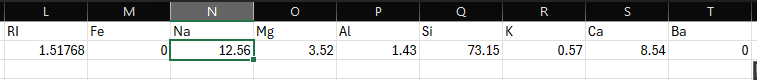
You could quickly set up a table like this:

Here, in cells M1, we write RI, and in cells N1:U1 we write the various elements listed in cells B1:I1. Now, in cell M2, we write the Refractive Index that we are to look up. In cell N2 we write the formula =XLOOKUP($M$2,$A$2:$A$215,B$2:B$215) and auto-fill this across until cell U2.

Example 2: Conditional Lookup

Now, what if your supervisor wanted you to make a glass sample with a Refractive Index 1.51768, but with no Fe. If we look at the table, the glasses in rows #30, and #32 both have the same refractive index but only #30 satisfied that criteria. This can easily be set up using the following formula:

=XLOOKUP(1, ($A$2:$A$215=$L$2)*($I$2:$I$215=$M$2),B$2:B$215)

Here, we set a return value of 1 as our first argument, and in our second argument, we effectively set up an AND function. By asking Excel to check for both conditions and returning only that multiplication of two TRUE values (1), we can extend the functionality of the XLOOKUP function.

Conclusion

The XLOOKUP function can be extended further by adding more AND, OR, or other logical operations. It is an extremely powerful function, especially when combined with interpolation, making it a valuable tool in various fields, particularly engineering and science.